DirectX 11
| Links:
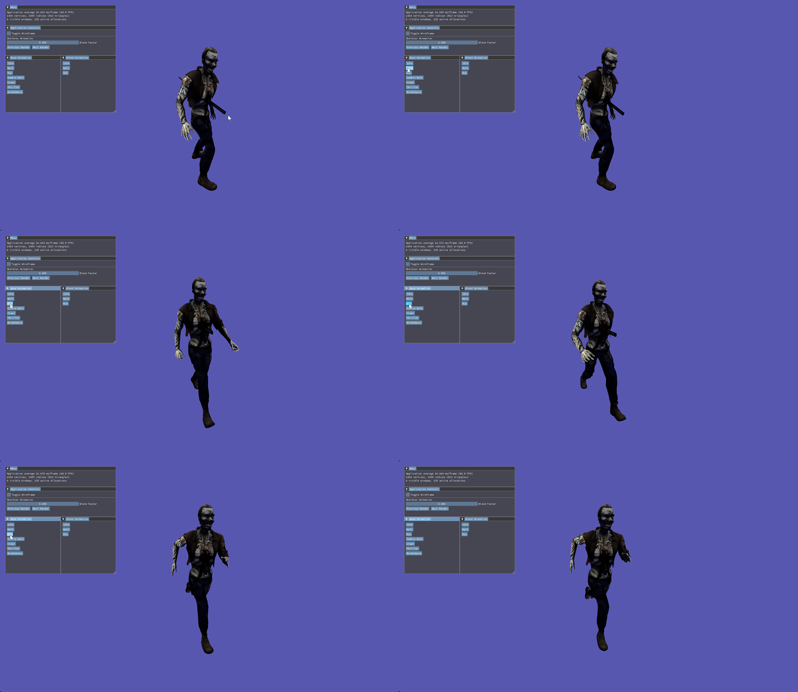
An endevour into low level graphics
DirectX 11 (DX11) marked my first serious venture into low level computer graphics, and it’s where I discovered my passion for working with graphics APIs. I’ve consolidated all my DX11 work here, along with technical details, as each project builds upon the last.
I had previously dabbled with OpenGL in a more guided university module that included significant hand holding. This DX11 project, was far more independent starting from just a basic triangle and expanding from there.
Fundamentals
For my first endeavour with DX11, I implemented several core features that would be expected in a basic graphics engine such as Phong shading, wireframe rendering, depth buffering, and billboarding techniques.
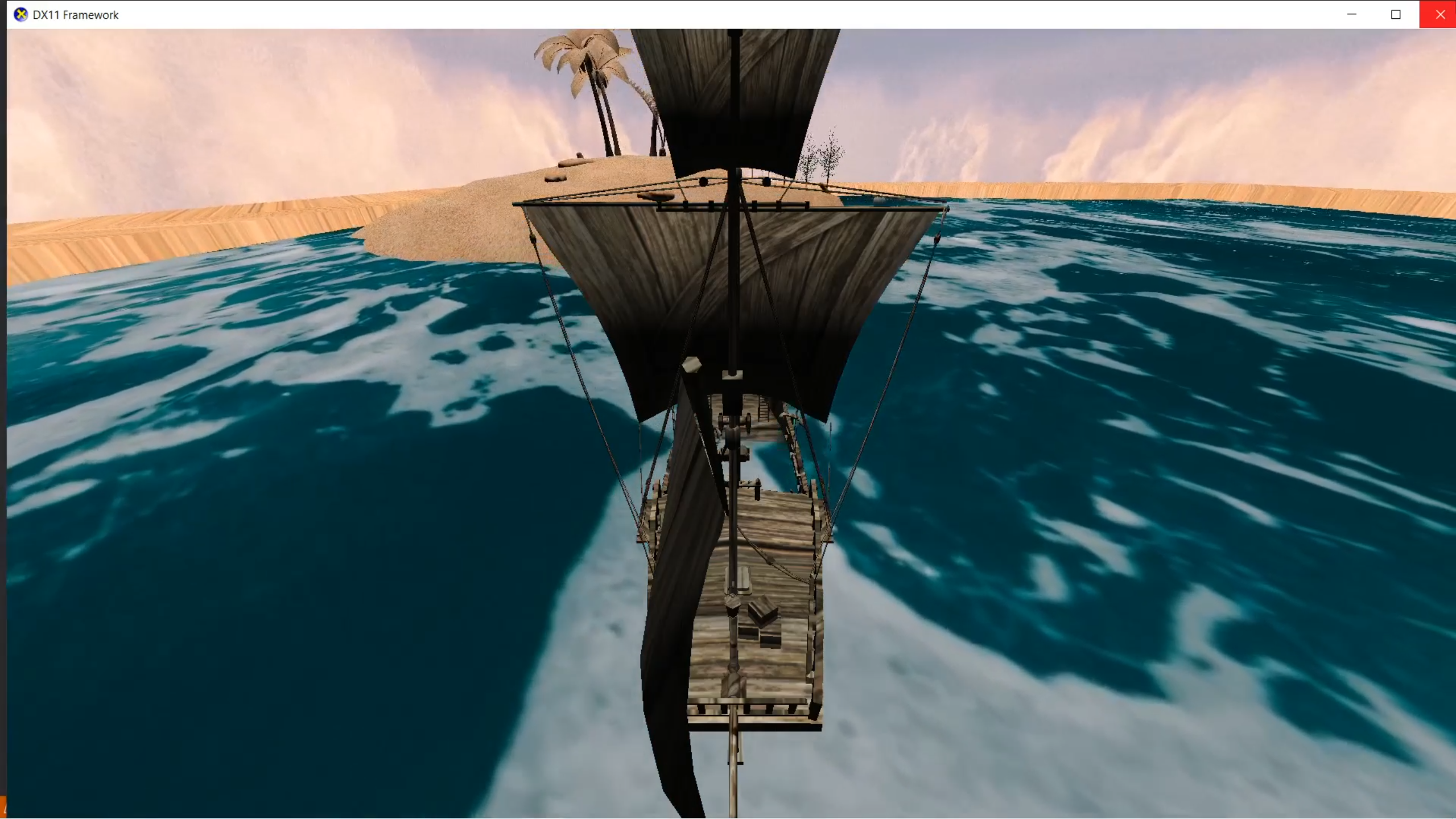
Looking back, these features seem relatively simple, but they were important milestones that mark my early progress in computer graphics.
Physics
The next project I undertook was building a physics system designed to work in tandem with DirectX 11. This was less about demonstrating rendering techniques and more about creating core systems and integrating them into an existing engine.
Each game object contains a Movement class, which includes all the functionality needed to respond to the physics engine. A custom vector class handles all the required mathematics for simulating physical behavior.
The physics system manipulates objects using velocity and acceleration, simulating effects like drag, collision, buoyancy, gravity, and torque.
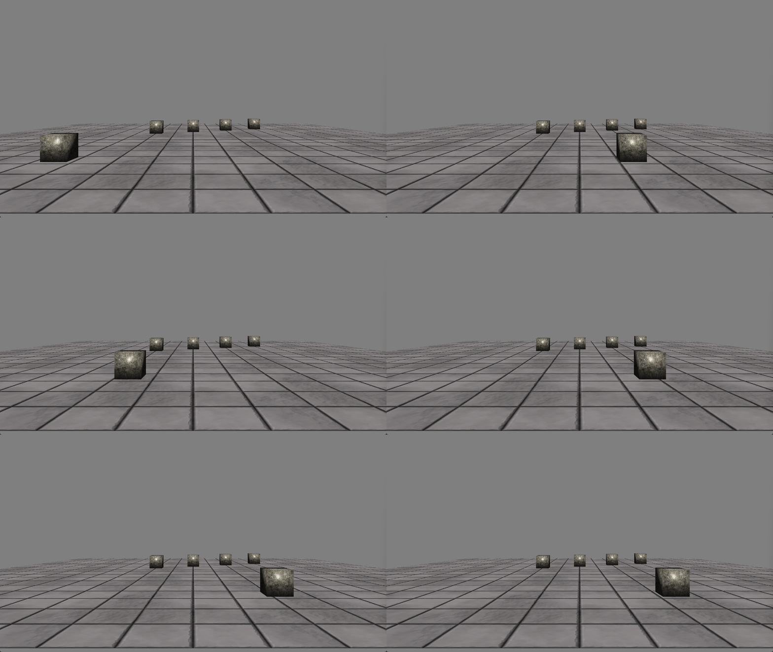
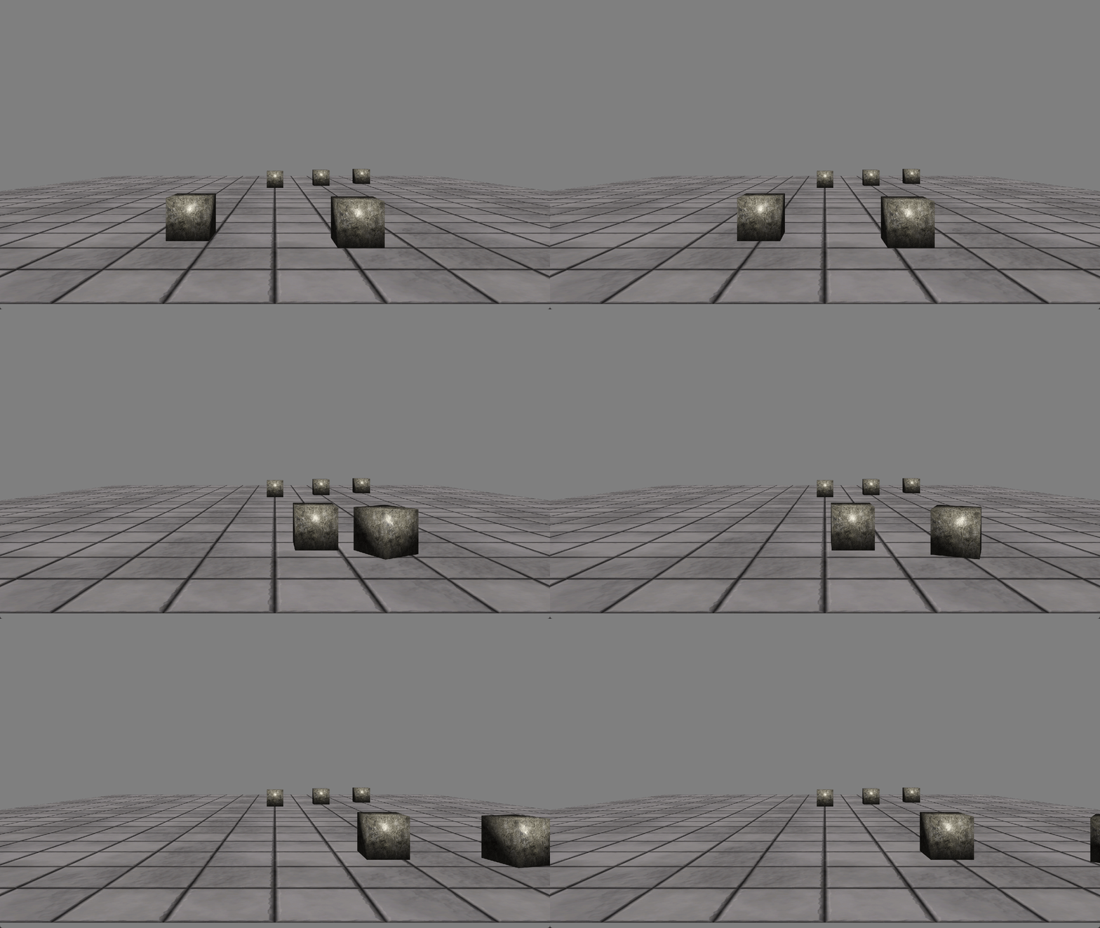
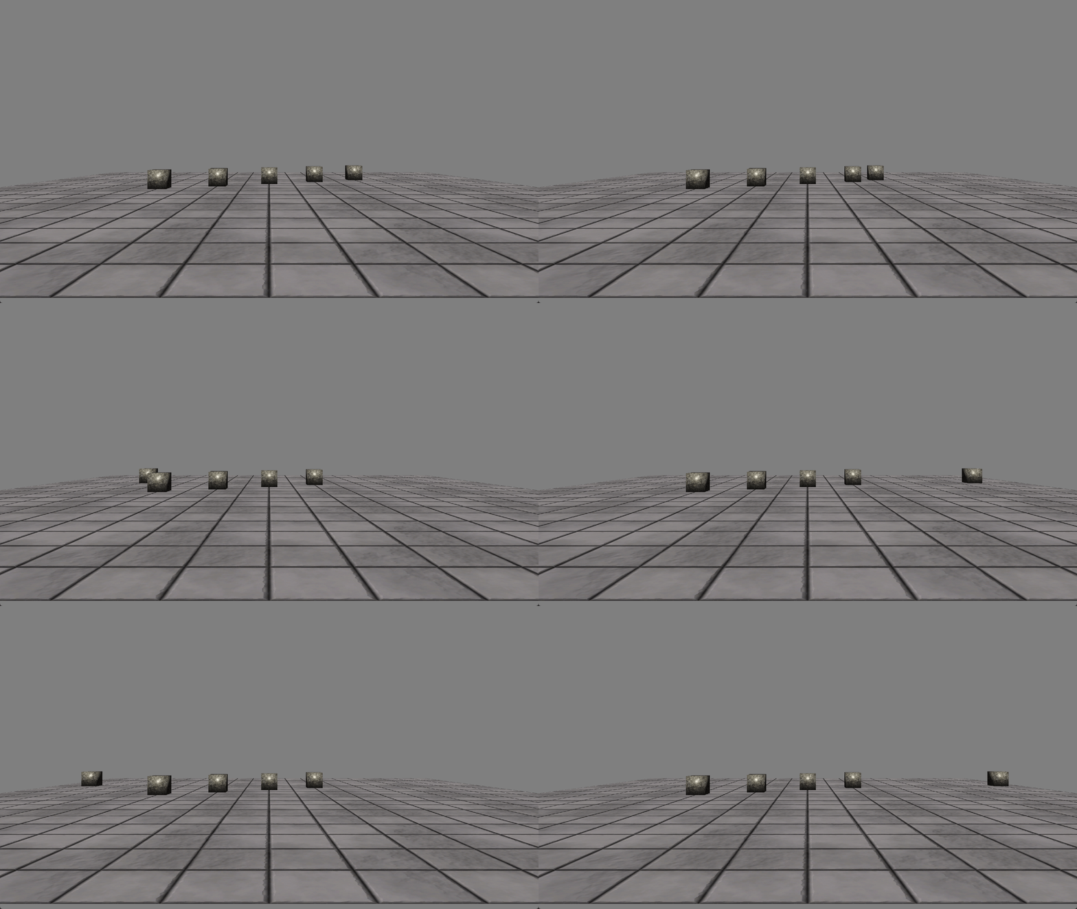
I also developed a particle system, allowing particles to be influenced by the physic system. This system was later extended with a 3D A* Pathfinding system that uses programmatically placed waypoints for dynamic navigation.
Advanced Rendering Techniques
After diving into physics programming for a while, I eventually came back to graphics programming. This time the project delved into rendering techniques that were more advanced than before.
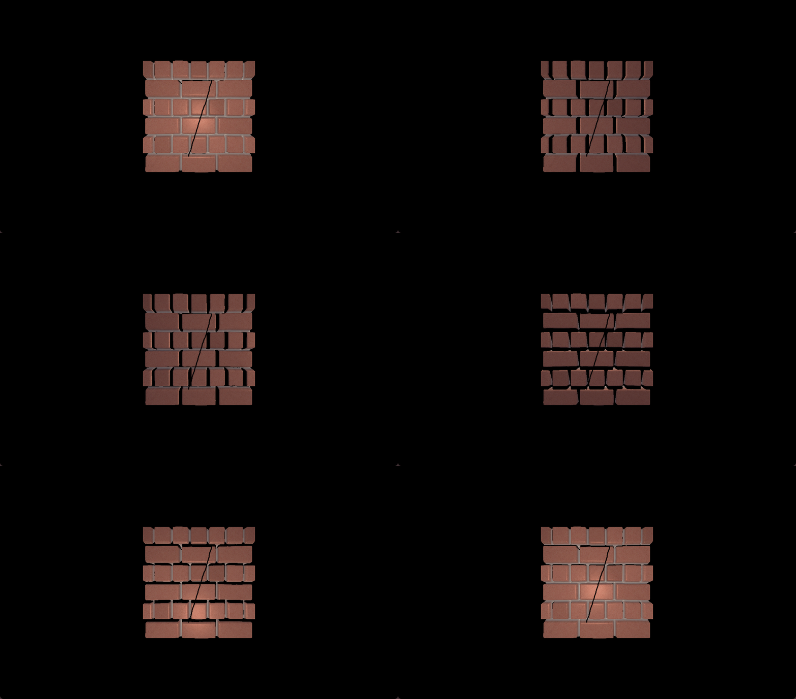
The first was normal mapping, which involved working with TBN (Tangent, Bitangent, Normal) matrices to simulate surface detail. Building on that, I added parallax occlusion mapping and self-shadowing.
These techniques significantly enhanced depth perception and surface realism.
The next technique developed was render-to-texture. This allowed for post processing techniques to be used, as the final render would be stored in a texture.
This enabled simple post-processing like colour modification. It also laid the foundation for more complex effects such as FXAA and colour correction.
This feature also proved invaluable when integrating ImGui, as it allowed me to visualise individual render buffers during deferred rendering.
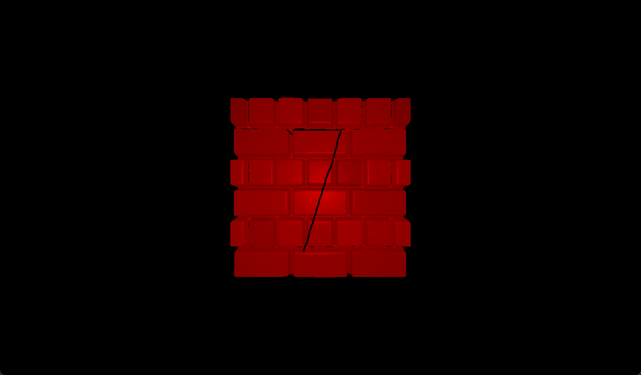
Deferred Rendering was the next big thing to move onto. The idea of deferred rendering is to mitigate redundant lighting calculations on overdrawn pixels. To do this you need to render the scene without lights then, output each element of the scene into a GBuffer. This contains Postion, Albedo/Diffuse, Normal, Emissive and Specular. It can be adapted to hold alternatives but, these are the standard.
Once the GBuffer is rendered out, the second stage of the deferred rendering can begin to calculate lighting for the scene. This offers no visual benefit but, allows us to have more lights within a scene as each light is only calculated for the pixels that are affected. It stops geometry having lighting calculated against the pixels it draws; when it could be obscured by another geometry call.
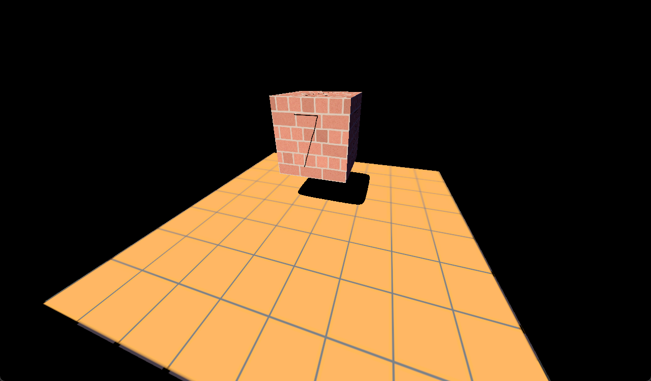
Finally, I implemented shadows. An integral element to realism, as lights that don’t produce them feel slightly otherworldly. Creating shadows depends on the light source and its style; sunlight vs a light bulb act differently in the real world so different techniques are needed. In the technique developed, a simple directional light is present which would be similar to sunlight. To recreate this, we render the scene from the lights perspective. It has a direction but, doesn’t necessarily have a point in space as its effectively infinite.
Though not perfect, due to various artefacts when moving the cube or light direction, it was a strong first attempt which I would correct in later projects.
Enhanced Rendering Techniques
Terrain is fundamental to allow a player to traverse a world. Sometimes, we want the experience to vary between playthroughs, which leads us to procedural generation (PCG). We have explored various methods for generating terrain procedurally. While some of these methods are now considered outdated, it is still valuable to understand alternative generation methods, as they can inspire or be incorporated into other generation techniques.
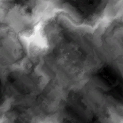
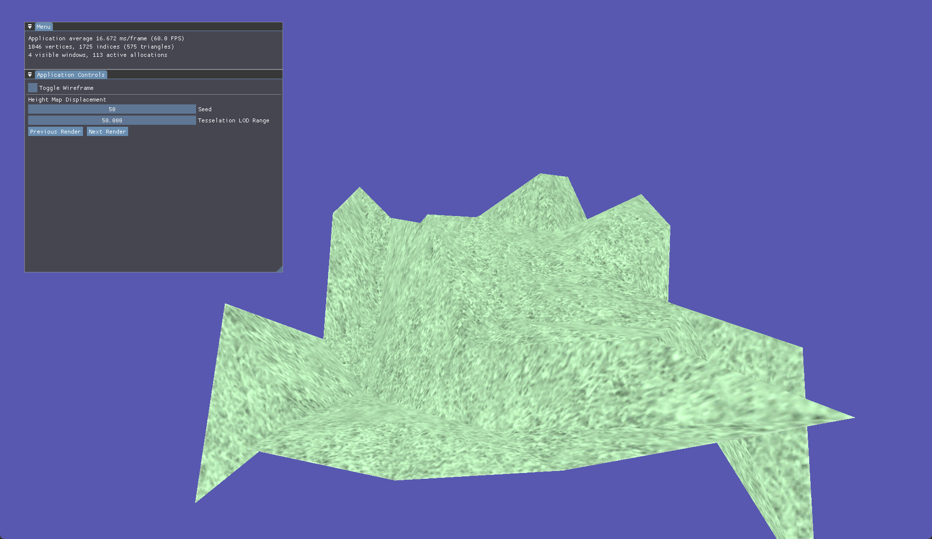
Some basic methods of terrain generation were the usage of displacement/height maps. Essentially loading in an image and using the values of each pixel to determine the displacement within the terrain. This can then be multiplied by a value to achieve the desired result.
| Displacement Map | Generated Terrain |
|---|---|
 |  |
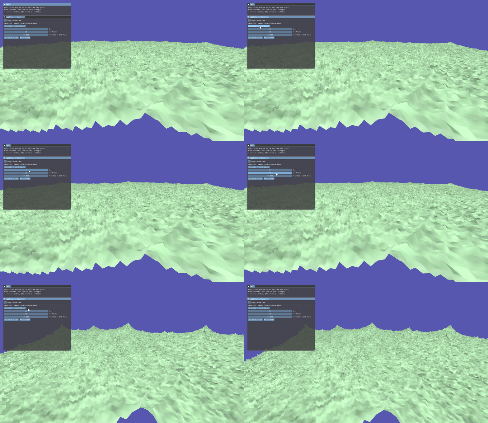
Going down the procedural route we started with Diamond Square, this method has you starting with a basic plane and a seeded value. In this case it was controlled via ImGui. Firstly, each corner is randomly assigned a value based on a roughness value, then a side length is calculated based on the plane size. After this has been done each corner is calculated using the side length then average to determine the midpoint which has its roughness shifted based on the seed and desired roughness.

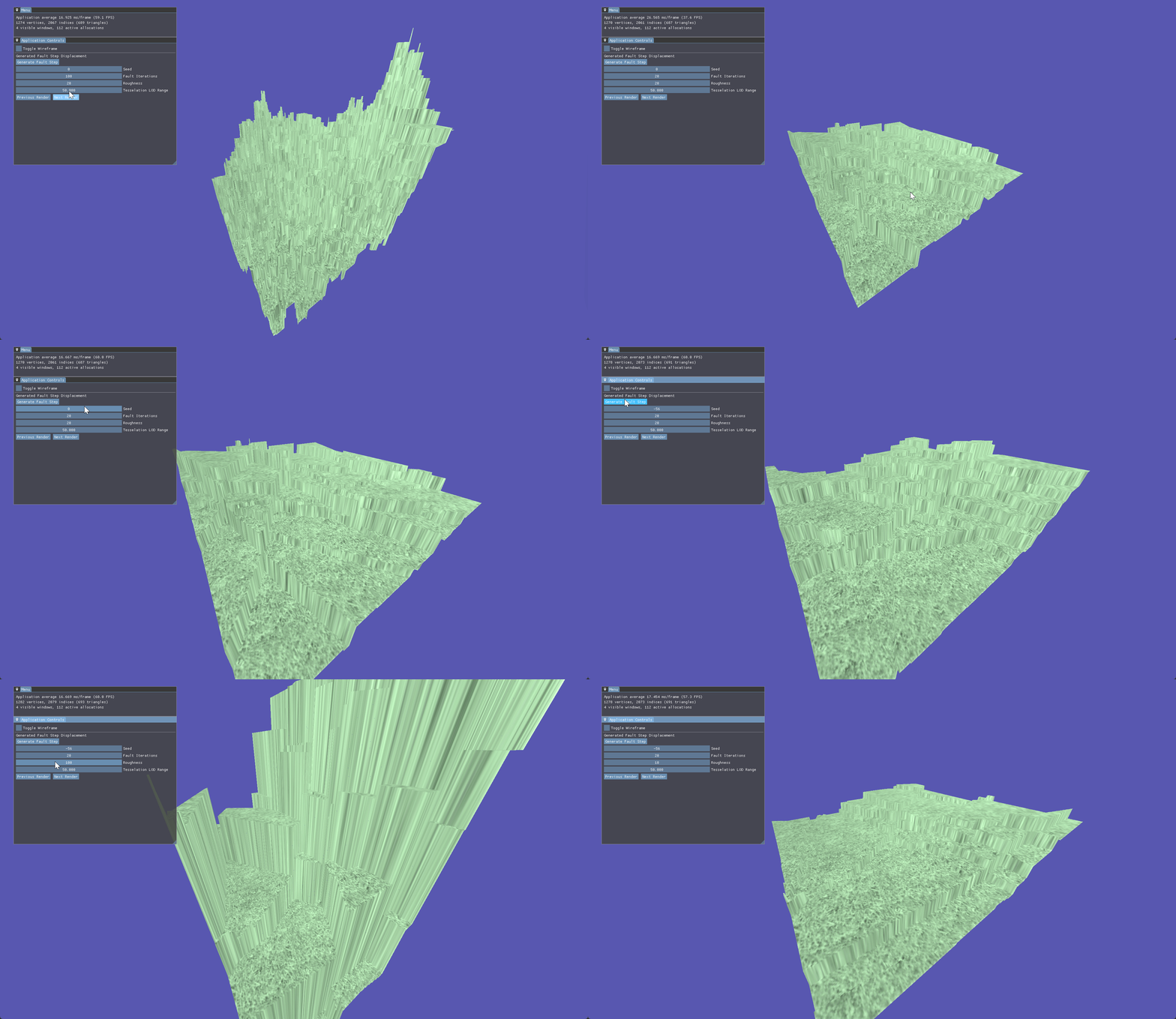
Then came the Fault Step algorithm. It is similar to Diamond Square algorithm due to also only needing a plane and ideally a seeded value. Essentialy, the Fault Step algorithm draws a vector across the plane then shifts the height of all vertices on one of the sides up or down. This happens for as many iterations as set by the user.
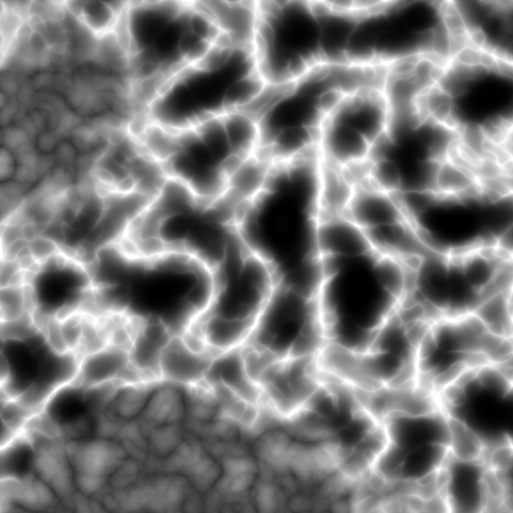
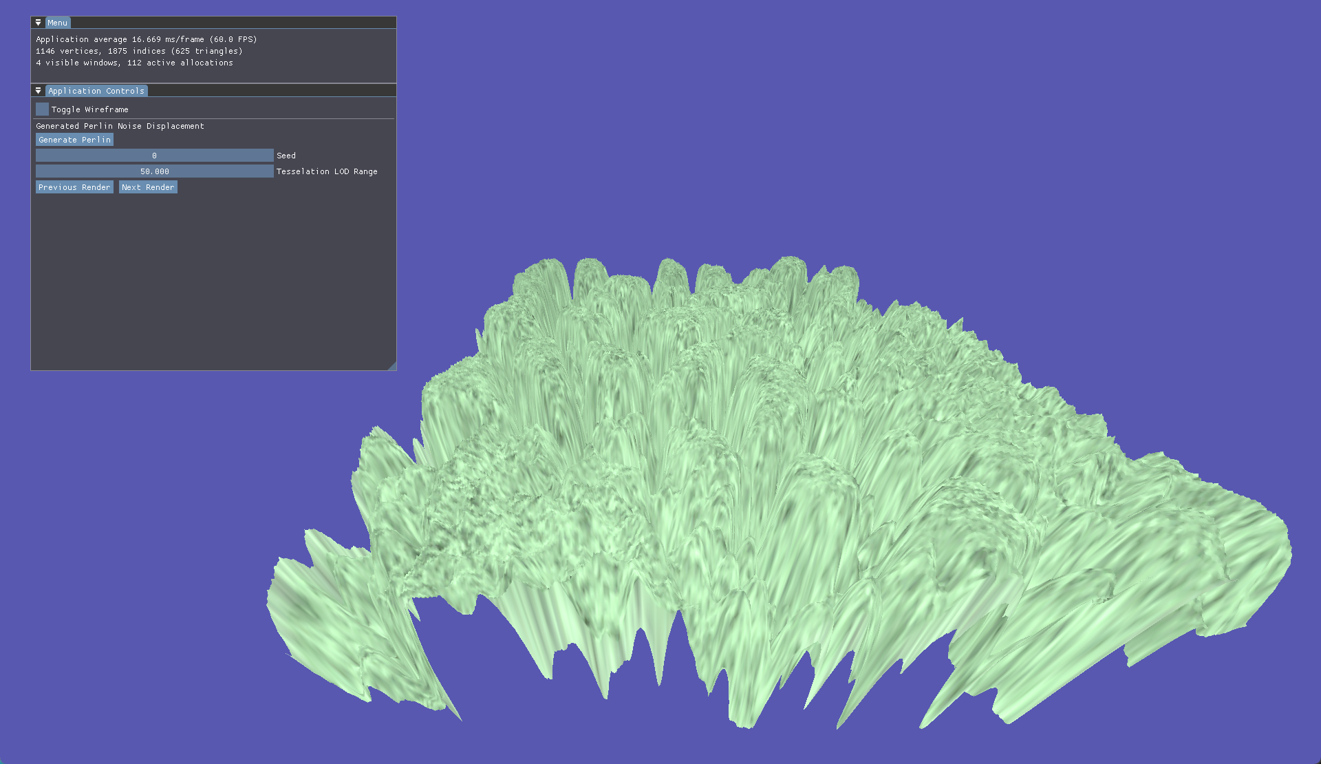
The last and most pivotal procedural generation is Perlin Noise. It builds from the previous setup used for a basic height map but instead of giving it a pre calculated height map, we generate the texture at run time.
Perlin noise allows us to tweak parameters such as octave and frequency to produce vastly different terrain types across generations. With our seed set to 0 we generate this perlin map resulting in this generated terrain.
| Perlin Map | Generated Terrain |
|---|---|
 |  |
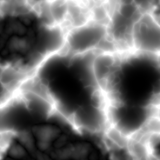
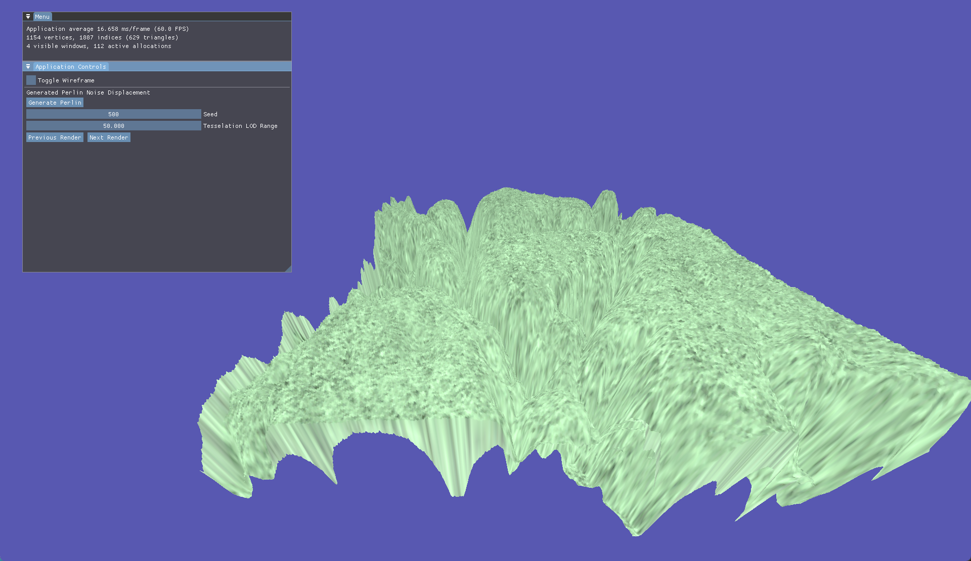
With our seed set to 500 we generate this perlin map resulting in this generated terrain.
| Perlin Map | Generated Terrain |
|---|---|
 |  |
With terrain being generated with various methods, we want a way to increase the polygonal resolution at runtime. To do this we turn to tessellation. We use further shader stages like hull and domain to calculate barycentric coordinates. Alongside this we use the camera’s position to dynamically tessellate based on camera distance.
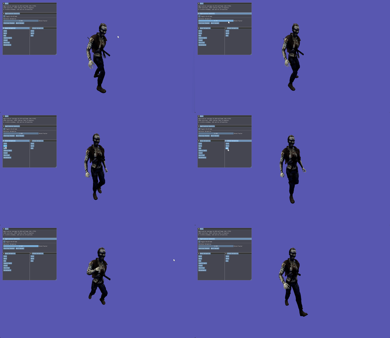
The final major feature I explored was skeletal animation, as part of this I learned how to skin, animate and blend animations for skinned meshes. Using Assimp to aid model and animation importing I built an animation class to read hierarchical bone and keyframe data. Bones are a quintessential foundation to how animations work. Each bone stores a position, rotation, scale for each key frame of an animation.
Within the bone class, each bone is updated via an internal update loop, which is called by the animator class. Within this loop a new translation, rotation and scale is determined based on interpolation of the current key frame to the next key frame.
Each frame the animator class will call UpdateAnimation, within this function CalculateBoneTransforms is called; if the animator has an animation set. Within CalculateBoneTransforms we start at the root node of the animation and work our way through the children updating each bone connected to the node, once updated we use the bone transform and multiply it by the parent bone transform then save this as global transform.
The next step is to find the bone made earlier when loading the model, this allows us to grab the offset for the specific bone then store the offset multiplied by the global transform. This is our final matrix that will be used in the shader. This happens for every bone within the animation, for every key frame.

Blending builds upon these foundations to allow a further interpolation between animations rather than just key frames within one animation. Using a weight factor we can blend one animation into another. By using the finalised bone matrix of each animation we can slerp between the transformation matrices. We then get the inverse blend of the first animation which reduces the effect of the first animation, whilst increasing the weight on the second animation. Once this is completed the global transformation is then a combination of the 2 bones interpolated multiplied by the parent transform. The process then continues as normal just like the update bone transform function before.
